Polyglot Persistence and friends

Have you ever noticed how a professional sketching artist uses multiple types of pencils for his work ? Each pencil has a different features and used to achieve different shades and details. The world of databases is very similar. You have many databases which specialize in different aspects of data storage and functionality and hence they provide you with additional use cases which others couldn’t have.

Polyglot persistence is a term used in the database community to describe that when using a database, it’s best to choose the type of database based on the usage and functionality. A standard example is of e-commerce companies. They deal with many different types of data. Storing all the data in one place, would require a lot of data conversion to keep the format same, which would inherently lead to a loss of information.

Historically, RDBMS databases have ruled the industry. But, necessity is the mother of invention. Though NoSQL databases have existed before, they never got a solid ground until the explosion of the web required companies like Google and Facebook to look for alternatives outside the classic relational storage realm. Now, NoSQL are ubiquitous in the time of big data.

Is there a metric to understand NoSQL distributed storage systems better ? The famous CAP Theorem. Also called Brewer’s theorem after Eric Brewer, the CAP Theorem provides a metric to classify and comprehend the attributes and limitations of NoSQL systems. It states that no distributed computer system can satisfy ALL of these three features:

• Consistency – every read would get you the most recent write
• Availability – every non-failing node will return a response
• Partition Tolerance – the system will continue to work if network partition occurs

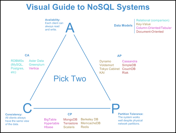
So, this means that all NoSQL databases can satisfy two out of these three features. Deciding which database to use comes down to the product requirement. Let’s cover some common databases belonging to different categories.

Cassandra

Cassandra is a database created by the folks at Facebook. It’s a column-family store. Column-family databases store data in column families as rows that have many columns associated with a row key. Column families are groups of related data that is often accessed together. A column family is analogous to a table in RDBMS. The difference is that you don’t need to have the same columns for all the rows. Other examples of such stores are HBase and Hypertable.

Cassandra is highly scalable. There is no single master, so scaling up is just a matter of adding more nodes to the network. Cassandra falls in the AP category. It’s designed to be high on availability and partition tolerance, but have the architects have to negotiate on consistency. It relies on a notion of eventual consistency. The data on a node, though not the latest now, will eventually be replaced by the most recent one.

Redis

Key-Value store. A hash table. A key-value store is a very simple NoSQL database with options for fetching, updating or deleting a value for a key. Redis supports storing lists and sets and can do operations like range, union, diff, intersection.

Redis is an in-memory store. This enables it to be a perfect option for high read and write rates, but limited to the size of data that can fit inside memory. Despite being a NoSQL system, it is difficult to grade Redis according to the CAP theorem. This is because it is generally used in a single-server deployment. One can create a Redis cluster using a master-slave scheme, but the behavior of it would depend on how it is configured. This blog post explains the functionality of Redis to great extent.

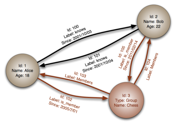
Titan

Titan is a graph database. Just like a graph, these databases have nodes and edges. The edges capture the relationships between node-like entities. Entities and relationships have properties.

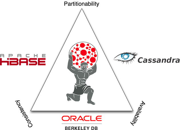
Titan is designed to support the processing of graphs so large that they require storage and computational capacities beyond what a single machine can provide. Titan supports Cassandra, HBase and BerkerlyDB as its backends. Their tradeoffs with respect to the CAP theorem are represented in the diagram below.

There is a fourth kind of NoSQL database, called document store. Expanding on the idea of a key-value store, document based databases store more complex data in the form of ‘documents’ as values assigned to a unique key. It’s most common examples are MongoDB and CouchDB.

References:

• Polyglot Persistence I
• Polyglot Persistence II
• NoSQL systems
• CAP Theorem I
• CAP Theorem II
• NoSQL Distilled: Book by Martin Fowler and Pramod Sadalage
• Graph databases Wiki
• Titan Official Docs

What is Spark ?

With the increasing amount of data at hand, there has always been development of ways to handle such large scale data, organize it, compute on it and ensure practicality. MapReduce is a revolutionary model which allows you to do data parallel computations on cluster machines while providing task scheduling, fault tolerance and load balancing. But there are some application where MapReduce falls short. According to the super famous Spark introducing paper by Zaharia et. al., such applications are those which use a working set of data across multiple parallel operations. This includes two use cases, iterative jobs (basis of most machine learning algorithms) and interactive analytics (SQL querying). Spark is a cluster computing framework which supports working on these cases, while providing all the benefits of MapReduce.

RDD

Resilient Distributed Datasets (RDDs) represent a read-only collection of objects partitioned across a set of machines that can be rebuilt if a partition is lost.

One can imagine RDDs as the backbone of Spark’s functionality which is simply a collection of objects distributed across clusters. Its fault tolerant and we perform various parallel tasks on the RDD. An RDD can be created by parallelizing a collection or by reading from an external source.

In general, there are two types of operations that can be performed on RDDs, transformation and actions. Imagine you have an RDD. A transformation is an operation wherein you transform the RDDs data into another form. For example a filter function which gives you the entries of the RDD with an even Id number. The tricky part is that Spark doesn’t actually perform a transformation on the RDD immediately. Instead it prolongs the task to a later time. This is called lazy evaluation.

Why would Spark behave lazily ? Imagine you called upon multiple transformations on an RDD, one after the other. Now Spark will create an directed acyclic graph (DAG) of these transformations. It will rearrange these tasks in order to optimize the execution flow and choose the best possible transformation path. Imagine you have map operation followed by a filter. Spark will rearrange these operations as filtering would reduce the amount of data undergoing a map operation.

The transformation tasks actually take place when an action operation is called. For example, when the user submits a Spark job for a collect operation, Spark will perform all the previous transformation tasks in the optimized manner, and send the results to the driver function. Also, RDDs can be cached at any time to persist the data in memory or disk. This is really handy when performing a long set of interrelated operations.

Driver and Executors

Driver is the main program which creates partitions, distributes and schedules tasks and manages the outputs of individual worker nodes. Executors are worker nodes’ processes in charge of running individual tasks in a given Spark job. Once the job is complete, they send the results back to the driver.

Spark Stack

Spark offers a whole range of integrated components which form the Spark stack. Spark SQL allows you to perform SQL-like data analytics on distributed data. With Spark Streaming, you can do real-time processing of live data streams. MLlib is the machine learning library providing most of what you’ll need for learning insights from the data on Spark. GraphX is Spark‘s API for graphs and graph-parallel computation.

The main selling point of Spark is how efficiently it manages data in the memory instead of the disk. This clearly doesn’t mean that ALL the data is stored in the memory. But Spark finds a way to organize the operations in parallel and optimize them, keep only the required amount of data in memory and manage the computations to provide greater performance improvements.

References

• Cloudera
• MapR
• StackOverflow
• EdX
• Spark Paper

A bit on recommendation systems

Recommendation engines are driving the internet. From suggesting us products on Amazon, movies on Netflix, to ads on Google and Facebook, no internet company is without recommendation systems. In this post I cover some basics of recommendation systems and some algorithms that power them.

The basic idea behind recommendations is using some inputs from the consumers and predicting a set of products back. This feedback that the engines receive is crucial. Explicit feedback refers to direct opinions of the consumer reflecting their choices and preferences. In case of movies this could be in the form of specific movie ratings by each user, for example (userId, movieId, rating). Implicit feedback is more subtle. This could be a user’s behavior over the internet, click rate, time spend on specific pages or page history. This can provide more intuition on the user’s patterns. Also its more readily available than explicit feedback.

Now, we will work with a sample case of movie recommendation system. This is based on the idea of collaborative filtering. Its concept is simple and very effective. Imagine Adam likes the movies X and Y. John and Maria like the movies X, Y and Z. So the system can suggest the movie Z to Adam. This is because Adam is more likely to share a similar movie taste with John and Maria as all liked X and Y.

Imagine we have a user-rating matrix X. This matrix has the user’s ratings for specific movies in every row. Similarly, each column has the ratings its received from different users. The idea behind learning user patterns is to factorize X into U and V, such that U captures user patters and V captures the movie patterns. Also, we want to select these two matrices such that the error for the users/movie pairs where we know the correct ratings is minimized.

If X is a m x n matrix, U and V will be m x k and k x n respectively. Here k is the rank of X. This is called low rank factorization. It helps in determining which factors control the observations. So, ultimately we are trying to get a hang of the user and movie matrices to better understand their patterns.

Now the question is, how to estimate such factor matrices. In order to learn those factors we need to minimize the following quadratic loss function:

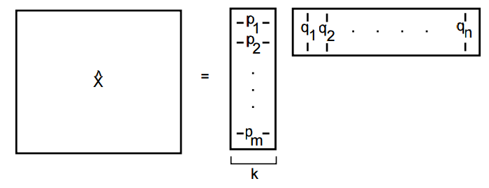
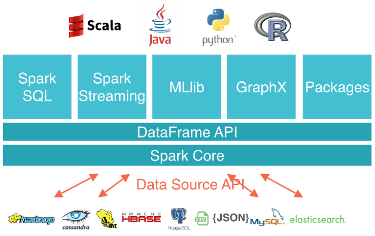
where is the observed ratings. One approach is to use Alternating Least Squares. If ‘fixes’ one of and , and minimizes the other. Then is ‘alternates’ by fixing the second one and minimizing the former. This alternation between which matrix to minimize is the reason of ‘alternating’ in the name. Clearly, we can add regularization terms to the loss function for better updates. Apache Spark’s MLlib has an implementation for ALS.

What the Boston Housing dataset taught me!

The Boston Housing Prices dataset was collected by Harrison and Rubinfeld in 1978. This dataset measures the housing prices against various factors which define the neighbourhood. The data consist of 506 observations and 14 independent variables. The variables are listed below along with their meaning:

1. crim – per capita crime rate by town.
2. zn – proportion of residential land zoned for lots over 25,000 sq. ft.
3. indus – proportion of non-retain business acres per town.
4. chas – Charles River dummy variable (= 1 if tract bounds river; 0 otherwise).
5. nox – nitrogen oxides concentration (parts per million).
6. rm – average number of rooms per dwelling.
7. age – proportion of owner-occupied units built prior to 1940.
8. dis – weighted mean of distances to five Boston employment centers.
9. rad – index of accessibility to radial highways
10. tax – full-value property-tax rate per $10,000
11. ptratio – pupil-teacher ratio by town
12. black – 1000(Bk – 0.63)^2, where Bk is the proportion of blacks by town.
13. lstat – lower status of the population (percent).
14. medv – median value of owner-occupied homes in $1000s.

Here, medv is the house price and is the response variable while others are predictor variables.

In this post I mention some statistical concepts I understood while playing with this dataset using R.

1. Multicollinearity

Imagine two or more predictors that are quite close to each other. Statistically speaking they are highly correlated. There is a substantial degree of linear relationship amongst them. The problem with this is that, when you have a strong correlation between your predictors, you can’t separately credit one predictor for the outcome variable. Essentially separating them becomes difficult, and that can impact your analysis of valuable (or redundant) predicators.

Following are the correlation values of the dataset. Can you spot the highly correlated predicators ?

rad, tax, indus and nox fall in this category. Probably their meanings also suggest the same.

There is a way to detect such predictors. This is done using a statistical concept called variance inflation factor. Correlated predicators increase the variance of the regression coefficients. This method calculates the inflation amount and helps in trimming those predicators out. Generally, a VIF between 1 and 5 is signifies moderate correlation, and  greater than 5 means significant correlation.

The difference in the two glm.fit is the presence of highly correlated predicators, which have been removed in the second one. The values of vif for each fit are consistent with the observation too.

2. Outliers

Outliers are the data points which (obviously as the name suggests) lie a little farther away from other points. The significance of outliers is their ability to manipulate the model estimates. It is always worth it to look for outliers, analysis and decide to keep them or exclude them.

These outlying points have an influence on the model. This influence can be summed up using two parameters. One, the difference between the observation’s value and mean 0f the predictor variable. This is called leverage. Second, the difference between then predicted value of that observation and the actual value. This is the distance.

Leverage is necessary for understanding how influential a data point is. Higher the leverage, higher the chances it will be an influential observation. It is very important to understand that influential doesn’t necessary mean that you can’t exclude the point. It just means that it can sway the regression line in its favour.

Cook's distance can be used to pin point observations which can be removed from the dataset. Essentially, this statistic measures how impactful a particular observation is. This is done by measuring the difference between the predictions of all values in the model, with and without the data point in question. An impactful data point can distort the accuracy and outcome of the prediction. Generally, an observation with a Cook’s distance vale greater than 1 is considered impactful. Also, some guidelines used 4/n or 4/(n-k-1) as a threshold, where n is the number of observation and k the variables.

 

This is the plot of cooks.distance(glm.fit2). This method is available in the car library in R.

3. Residuals

This is a simple concept. It is the difference between the predicted values and the observed values. But analysing them gives us a big edge. A very common way is to use various residual plots. (Warning: big white plots ahead !! :P)

The concept behind residual analysis is that the residuals shouldn’t be following a pattern. The residual errors should be approximately normally distributed.

The residuals are randomly scattered. This means linear regression works fine for this dataset. Instead, if we get a plot which forms a non-random shape (like a U or an inverted U) then we need to look more closely into our model (or maybe try a new one, or maybe clean the dataset a bit).

These graphs show that the residuals are normally distributed.
This is the code for the above graphs.

plot(glm.fit2$fitted.values,resid(glm.fit2),xlab='Fitted Values', ylab = 'Residuals')
abline(0,0)
plot(density(resid(glm.fit2)))
qqnorm(resid(glm.fit2))
qqline(resid(glm.fit2))

Thank you for reading. Bye.

---

References:
http://support.minitab.com/en-us/minitab/17/topic-library/topic-library-overview/

Click to access R7.pdf

http://onlinestatbook.com/2/regression/influential.html
http://blog.minitab.com/blog/adventures-in-statistics/why-you-need-to-check-your-residual-plots-for-regression-analysis

Functional Programming: Basics 1.0

Functional Programming (lamely referred here as FP) is super-cool. This blog post is a short intro to FP and covers some basic elements of FP with Scala. The aim is to write about some features which are imperative for writing good functional code. Scala is a functional as well as object oriented language. Its different facets fit together to ease the pain of writing cryptic functional code (it can still get pretty obscure!).

1. Pure Functions

Must not have heard that before! So, FP is all about pure functions. Its basically writing your entire programs as functions (hence the name), and these functions have to be pure functions. So what is it ? Its a function with no side effects. That is the definition, but we hardly expect to make sense of that. Simply, a side effect is anything that the function is doing other than returning the desired result.

In imperative programming, we write so many such functions. Imagine a function that reads from a file, updates the data structure, prints to the console and finally returns the result. All of that are side effects (expect returning). So how could one manage it without them. FP does manage. Its not that we won’t be doing all that stuff. There is a restriction on how we write our programs, not on what programs can express.

Pure functions can be understood with the help of the concept of referential transparency. The idea is simple, sum(1,2) will always give 3, no matter what. So we can replace the former with 3 everywhere in our program. So for referential transparency, the expression can be replaced by its result without changing the meaning of the program. And the function is pure if calling it with referential transparent arguments is also transparent.

So this means we’ll be writing (pure) functions in FP that precisely know what to do (no side effects), are exact in their definition, are reusable, can be replaced like expressions in algebra, and can be parallelized too.

2. Higher Order Functions

Functions in Scala are first class values. They are the dudes. They can be passed as arguments to other functions, have other functions inside them, can be assigned to variables, and much more.  Its best to demonstrate this with some examples.

//
// A 'map' function - a higher order function
def map(f:Int => Int, v:Int):Int = f(v)
def square(x: Int):Int = x*x
def cube(x: Int):Int = x*x*x
println(map(square, 2)) // 4
println(map(cube, 2)) // 8
//

So, here ‘map’ is a function which takes in a function as its first parameter, and a value as its second parameter, and returns the applied parameter function to the value. f:Int => Int refers to a function taking in Int and returning Int.

//
// A 'multiple_by_x' function - a higher order function
def multiple_by_x(x:Int):Int => Int = { n:Int => n*x }
val multiple_by_2 = multiple_by_x(2)
val multiple_by_3 = multiple_by_x(3)
println(multiple_by_2(2)) // 4
println(multiple_by_3(2)) // 6
//

 Here, a function is returning a function. multiple_by_x takes in x, and returns a function which multiples x to its parameter. This way multiple_by_2 is a function which always returns us a multiplication of 2.

This covers the two most important properties of higher order functions, having functions as arguments, and returning functions as its results.

3. Lazy Evaluation

This is what the name suggests, i.e. postponing the evaluation for a later time (also called non-strict evaluation). This indeed changes the order in which the program would execute. But since we are talking about FP here, everything is written in a modular fashion. So a change in order shouldn’t matter. More importantly, lazy evaluation provides performance benefits by delaying needless calculations for a later time (when they are required). Also, it provides the ability to construct potentially infinite data structures.

//
val x = {println("foo"); 10}
println("bar")
println(x)
//

This prints, “foo”, then “bar”, and finally 10.

//
lazy val x = {println("foo"); 10}
println("bar")
println(x)
//

 This prints “bar”, “foo”, then 10. This is because x is defined as a lazy val, and hence is called in use, only when required (Ref). This helps in stalling evaluation of recursive calls to such a time that its necessary (see Streams).

This wraps up this one! I aim to add more advanced features in further posts. Ciao!

Autoencoders and Dimensionality Reduction

This post is aimed at folks unaware about the ‘Autoencoders’. Some basic neural network knowledge will be helpful, but you can manage without it. This post is an introduction to the autoencoders and their application to the problem of dimensionality reduction.

What are autoencoders ?

These are an arrangement of nodes (i.e. an artificial neural network) used to carry out a straightforward task, to copy the input to the output. The input that is given in, is transformed to a ‘code’, and then the input is again reconstructed from this ‘code’. Weird right ? No. The catch is that this conversion from the input to ‘code’ and then its reconstruction allows the autoencoder to learn the intrinsic structure of the inputs. Basically its learning your inputs, and without any labels (unsupervised learning).

Technically, an autoencoder takes an input x and maps in to the internal representation y.

Here, W is the weight matrix and b is the bias. The vector y is the hidden representation or the ‘code’ and is then again transformed to recreate the inputs.

W’ and b’ are the weight and bias matrices. The function s in the above equations is the function of the nodes. The most common one is the logistic or sigmoid function. The point is to have the transforming function as a non-linear one like sigmoid, tanh, etc. I’ll get to the logic behind this soon.

This image should help in consolidating a mental picture of what you read above. So, you can imagine an autoencoder as and encoder + decoder. The input layer + hidden layer (the one in the middle) perform the role of encoding the input to an hidden representation. The hidden layer + output layer do the job of undoing the encoding, that is decoding. The weight matrices give the weights of the connections between each nodes of a different layers. The training of the autoencoder is nothing but adjusting the weights such that the reconstruction error is minimised.

What’s this error thing ? This error can be measured in many ways, mainly to account for the distributional assumptions on the input given the code. The most common one is the least squared error, another important one is cross-entropy error. Its nothing but a fancy term for how different the reconstructed output is from the inputs.

And how do you expect to train the autoencoder ? Oh you mean adjusting the weights! Thats where the mystical backpropagation algorithm comes in. 🙂 You may take some time get you head round this one, so don’t panic if you get lost in its derivatives and gradients. By the way, thats not the only way, but certainly an important way.

What has an autoencoder to do with dimensionality reduction ?

Dimensionality reduction is a huge topic. You can find loads of material on it. Basically, its reducing the dimension of the input data for better analysis, better visualisations and hence an overall better understanding of the data. You can’t underestimate how important that can be.

But don’t we have loads on dimensionality reduction algorithms ? Absolutely! There is the classic PCA which probably we all start with. But the autoencoder beats the PCA (I’m not propagating replacement of PCA with the autoencoders).

If you haven’t realised it yet, the autoencoder is reducing the dimensions of the data by transforming the input into the ‘code’ layer (the middlemost hidden layer obviously has lesser nodes than the input layer). And given enough depth and better training, the autoencoder does a pretty good job at capturing the essential statistical knowledge present in the input data. Also, the autoencoder uses a non-linear function and is able to gather more, unlike the PCA (which is a linear algorithm, and may not be able to cater to the intricacies of all types of datasets).

What the earlier figure showed was a simple three layer autoencoder. With a linear function, it does no better a job than the PCA. It learns the hidden layer as a linear function of the data with the least squared error minimized, which is exactly what the PCA does. Now look at the next figure!

Instead of having just one encoding and decoding layer, you can have multiple layers doing  each of the role. This is what I meant by depth. The resulting autoencoder is called a stacked autoencoder. And now if you throw in an unsupervised neural network model to further tweak the layers’ weights before fine-tuning them by backpropagation, you get better training.

---

If you go ahead and take a course on deep learning and neural networks (or atleast go through my hyperlinks and references), you’ll soon realise that all these models are nothing but mathematical equations. Its quite fascinating what mathematics can do!

I want to try the concepts of stacked autoencoders with better pre-training and test them against images. Lets see, hopefully in the next post!

I hope I managed to bring neural nets (or machine learning) to the attention of some folks! Thanks !

---

Further reading / References:

• http://deeplearning.net/tutorial/dA.html
• http://alexminnaar.com/deep-learning-basics-neural-networks-backpropagation-and-stochastic-gradient-descent.html
• http://deeplearning.net/tutorial/SdA.html#stacked-autoencoders
• http://www.cs.toronto.edu/~hinton/science.pdf

---